Network decomposition 3: Centralized construction

20 Apr 2020

This is the third post of a series on distributed network decomposition. The introductory post of this series is here. This post explains how to build a network decomposition in a centralized manner. As a consequence it also shows that such decompositions exist with nice parameters.

Recap of previous episodes

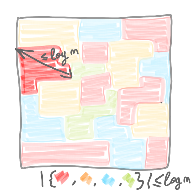
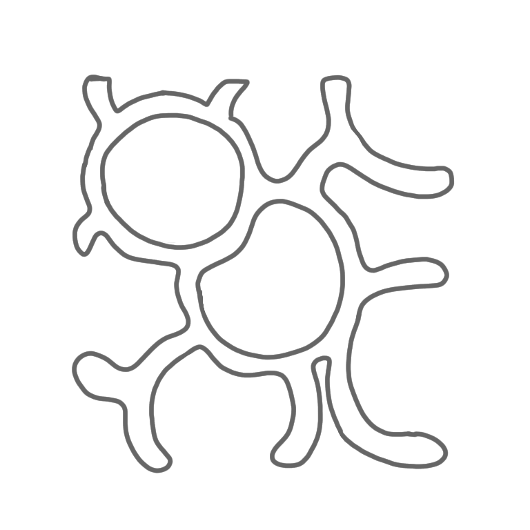
In the previous posts we saw how network decomposition can be useful to build efficient local algorithms. Such algorithms are efficient only if the network decomposition has good parameters, that is a small number of colors, and a small diameter for each component. We won’t bother with multiplicative constants, or even constant exponents, so let’s say that basically, we look for something like in the following picture, with $\log n$ colors, and $\log n$ diameter.

Basic technique to get a coloring

Suppose you want to compute a coloring in a graph in the most simple way. You can start with the first color $c_1$, pick a node $v$, put color $c_1$ on it, then choose a second node that is not a neighbor of $v$, put again color $c_1$, and so on and so forth, until you cannot use color $c_1$ anymore. Then you take color $c_2$, and repeat the process, considering only the nodes that do not have color $c_1$, etc.

This is basically repeating an algorithm for MIS we mentioned in the post about local algorithms.

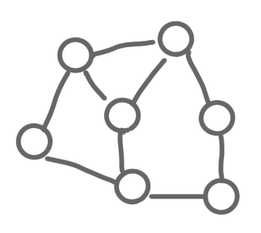
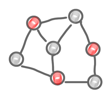
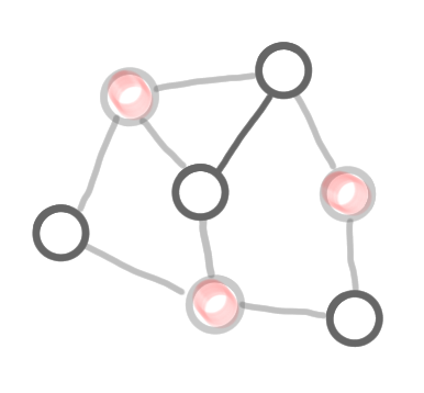
Step by step construction of a coloring. (1) The graph, (2) the result of the computation of the first color class (exactly as in the MIS algorithm), with the frozen nodes in grey, (3) the remaining nodes and edges after deletion of the colored nodes, (4) second color, (5) third color, and (6) the computed coloring.

Adapting the technique to network decomposition

We adapt the technique from the previous section to network decomposition. That is, instead of picking a node and coloring it, we pick a node, and color the ball of radius $\log n$ around it. Similarly to what happens in the coloring algorithm above, every time we color a ball, we freeze all the nodes that are adjacent to it. That is, they will not be considered any more for the color at hand. Once we are finished with a color, we go to the next color, remove the nodes of the previous colors, defreeze the frozen nodes, and start again.

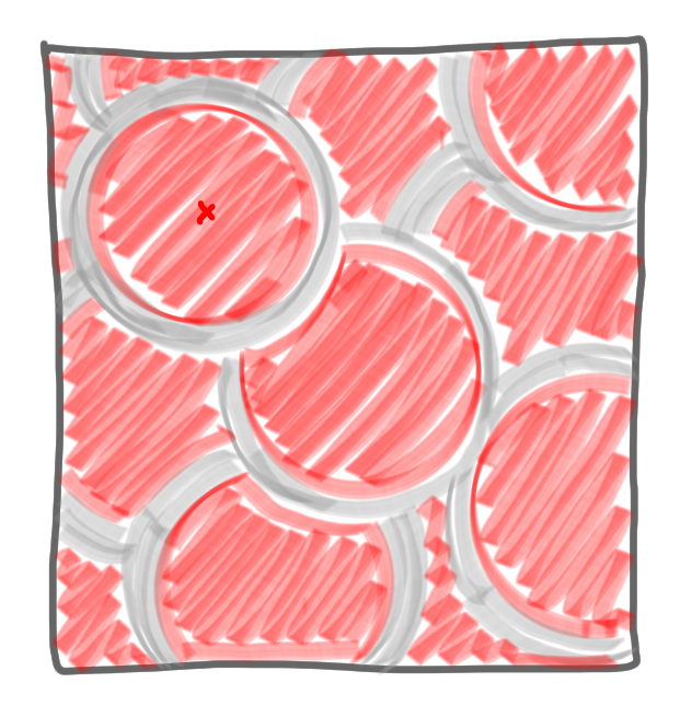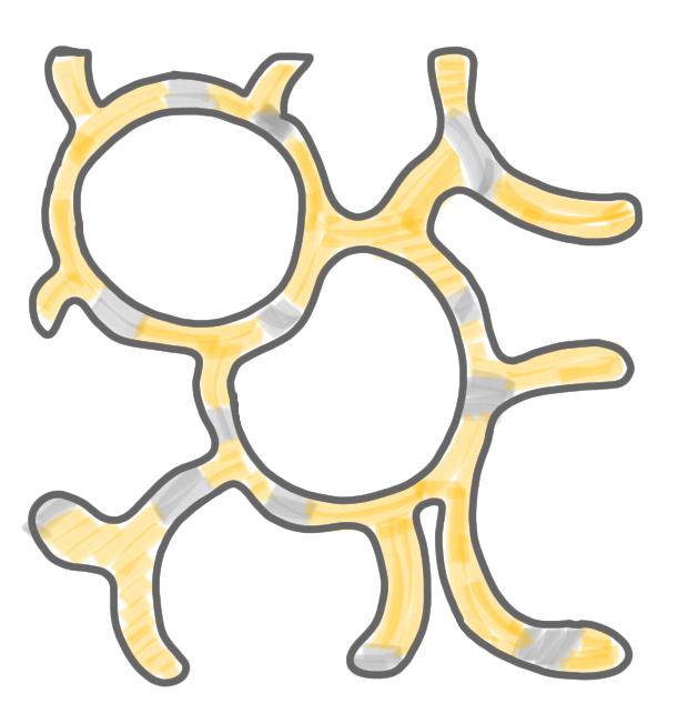
Computation of the first color class: (1) choose a node, and select all the nodes at distance at most $\log n$ from it, (2) freeze all the nodes that are adjacent to a selected node, and (3) repeat the operation until all nodes are either selected or frozen.

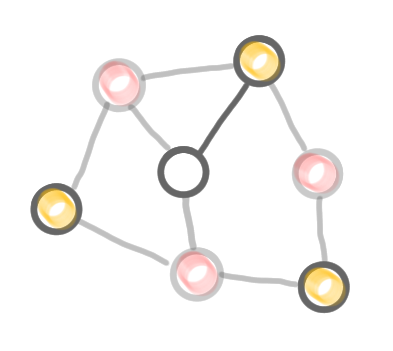
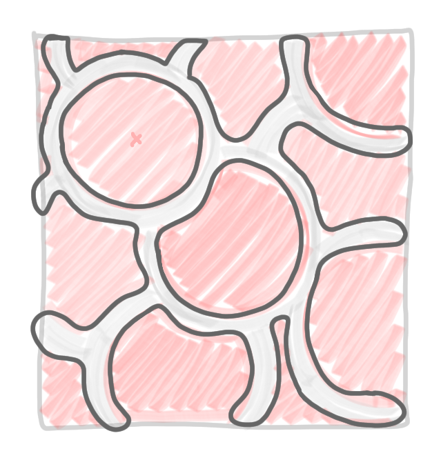
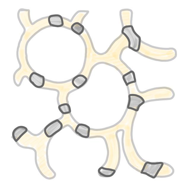
Computation of the second color class: (1) and (2) remove all the nodes of the first color class, and defreeze all frozen nodes. (3) Run the same procedure as for the first color class.

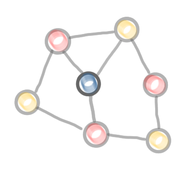
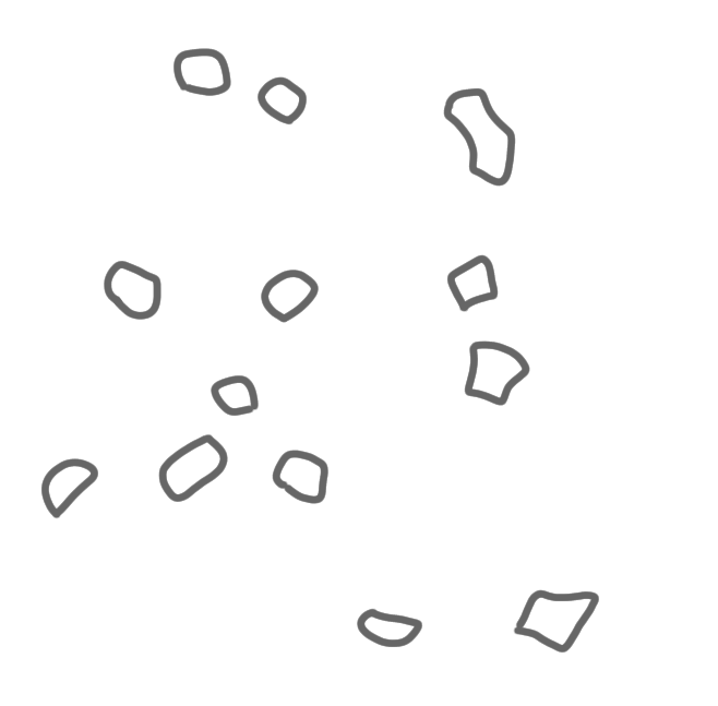
Computation of the third color class: again, (1) and (2) remove all the nodes of the previous color classes, and defreeze all frozen nodes. (3) Run the same procedure as for the first color classes. Now all nodes are selected, thus the algorithm stops.

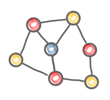
The network decomposition produced by the algorithm.

An unbalanced coloring

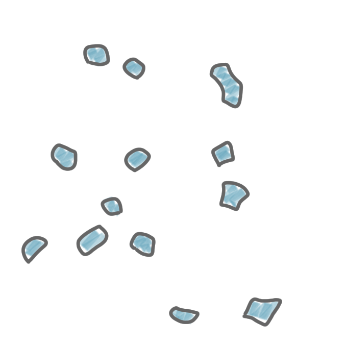
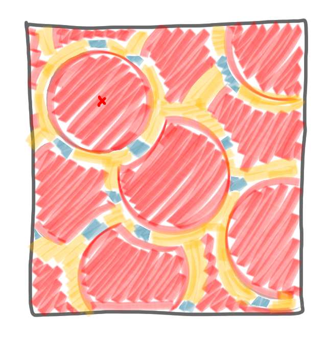
The first thing one can note on the picture above is that the decomposition is not balanced at all: a huge part of the network is red, a small part is yellow, and a tiny part is blue. That might look like a bad thing, as for algorithms having balanced decomposition is usually a nice feature. But actually this is not a problem for the algorithms built on a network decomposition, as presented in the previous post. And, in fact this imbalance is good for us. Indeed suppose that each color covers at least half of the remaining nodes, then after at most $\log n$ steps, all nodes are colored. This, in turns, implies that the number of colors is logarithmically bounded, which is what we were looking for.

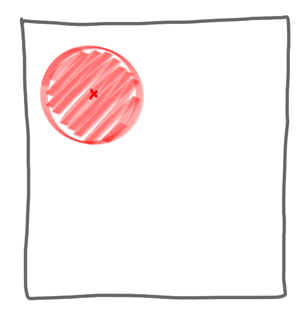
But, is this always the case? No, you can have a situation like the one on the following picture: you pick a node and in its $\log n $ neighborhood, there are very few nodes, but the number of nodes that is frozen at the border is huge. If this happens everywhere, the number of nodes colored by a the first color class is not a constant fraction of the total number of nodes.

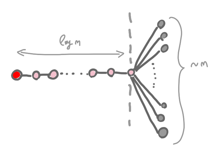
Therefore, a bad situation for us is when the ratio between what is inside the ball, and its border is small.

We could try to show that we can choose the centers in a smart way to avoid this behavior, but it wouldn’t help much with the distributed construction that follows, as such a smart choice could require a large view of the graph. Instead we control the size of the balls.

Growing a ball

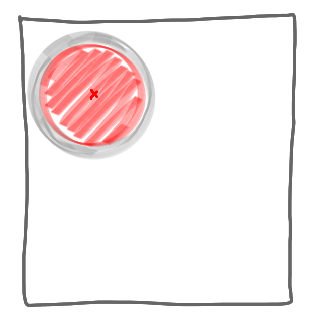
A technique to ensure that the interior/border ratio is large is to build the ball around the selected center in the following way, called ball carving.

Start with only the center
Iterate the following:

Measure the number of nodes in the border
If it is at least twice the number of nodes in the ball, take all these nodes in the ball, and restart the loop.
Otherwise leave the loop.

Freeze all the nodes of the border.

Note that the loop can be run for at most $\log n$ iterations, as otherwise the ball would contain more than $n$ nodes. Thus the balls built this way are ok with the definition of the network decomposition.

By construction, the size of the border of the ball is at most the size of the interior of the ball. That is, if we select $m$ nodes to be in the ball, we freeze at most $m$ new nodes. This is enough for the whole construction to work.