Network decomposition 4: Weak and strong decompositions

05 May 2020

This is the fourth post of a series on distributed network decomposition. The introductory post of this series is here.

In this post, we take a look at the different versions of network decomposition (weak and strong), and how we can go from one to the other.

Recap of previous episodes

In the previous posts, we saw what a network decomposition is, why it is useful to the design of local algorithms and how we can build such object with a sequential algorithm. Before we describe the distributed efficient algorithm (that is the core of series), let us give a further look at two different types of decompositions.

What is the diameter of a component?

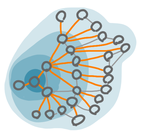
In the second post of this series we defined network decompositions, saying that the connected components of each color class have diameter at most $d$. As usual, the diameter is the maximum over all pairs of nodes of the minimum length of a path between these two nodes. But which edges can you use for these paths: only the edges of the subgraph, or all the edges of the graph? The first way defines the strong diameter and the second is the weak diameter. These can be very different, as pictured below.

On this graph, the blue component has weak diameter 2 and strong diameter 9.

The distributed algorithm we’ll study builds a network decomposition with a logarithmic weak diameter.

Going from strong to weak diameter

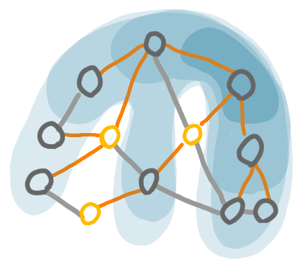
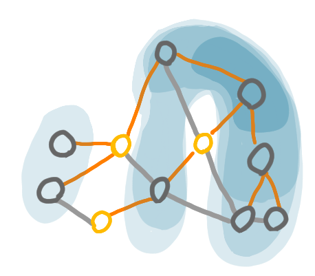
For some applications it might be better to have a strong decomposition, and the algorithm provides only a weak one. This is not a big problem. The paper of Rozhon and Ghaffari provides a sketch of the known approach to builds a strong decomposition with $O(\log(n))$ colors from a weak one with also $O(\log(n))$ colors. It is even simpler to have such a transformation if we just insist on having polylogs: take your weak decomposition, make the nodes of each component act like in a centralized algorithm (by gathering the whole topology of the component and simulating), and make them compute a strong decomposition of the component itself. For example, take a component of weak diameter $O(\log(n))$ with color yellow; these yellow nodes compute a a strong network decomposition of the component, and now the nodes have $\log(n)$ shades of yellow. In total this makes a strong decomposition with $O(\log^2n)$ colors.

The first picture is a weak decomposition with two colors, yellow and blue. Note that the strong diameter is large in comparison with the weak diameter. Now, if the yellow component "strongly decomposes" itself, we get three shades of yellow, and the new yellow components have small strong diameter. We can do this for all components of all colors classes, in parallel.

We finish this post with some technical aspects of weak decompositions.

A tree to keep track of the diameter

Remember that for the centralized construction, we create the component by making the balls grow layers by layers. Now suppose that we would build a spanning tree of the component as we go: at each new layer, we would wire the nodes as leafs of the tree. The depth of this tree is between half the diameter and the diameter.

The nodes of a component, added layers by layers, during the growth of a ball, for the centralized construction. The orange edges are the edges of the tree, the gray edges are other edges of the component. The diameter is 5, and the depth of the tree is 4.

In the distributed network decomposition, some balls will grow in a similar fashion as in the centralized algorithm, but then they will be modified. In particular some nodes will leave the component. Also, as we want the tree to have a depth that bounds the weak diameter, this tree may have to use edges that are not within the component. Hence we use a Steiner tree using the edges and nodes that may not be in the component.

The blue patches show the balls of various distance from the root, using the nodes and edges of all the graph. In particular the yellow nodes are not part of the component, but they are used by the tree.

Giving up the connectivity

Actually now that we measure the diameter via the tree, we can consider non-connected components.

This change in the definition useful in the distributed algorithm as we don’t want to keep track of whether the component is connected or not.