Network decomposition 2: Impact on distributed algorithms

10 Apr 2020

This is the second post of a series on distributed network decomposition. The introductory post of this series is here. This post explains why network decomposition is useful.

Recap of previous episodes

We saw in the first post of the series that one can simulate the greedy centralized algorithm in the local model, by using the identifiers as a schedule, but that this was horribly slow. We also looked at an algorithm that gathers the whole topology of the graph, this will be useful here.

Everything is easier with a coloring

It is easy to see how we could use less time steps to run the greedy algorithm: if you have two nodes that are far enough one from the other, you can select both without running into trouble. And then instead of two, you can select a large number of nodes, as long as they are far away one from the other. This way in one round you can select and de-select a lot of nodes.

Now, more generally, imagine that a mysterious friend gives you a (proper) $k$-coloring of the graph. You can use it to parallelize the algorithm the following way. First, pick the first color, select all of its nodes, de-select all the nodes adjacent to these nodes. This cannot create a problem as the nodes of a color class cannot be adjacent. Then continue by doing the same with the nodes of the second color that are still active. And so on and so forth, until you have considered all the colors.

This algorithm basically takes $k$ times steps, which is awesome if your mysterious friend gave you a 10-coloring.

Now there are two problems:

1. You do not have a mysterious friend, and computing a good coloring yourself might not be easier than computing the MIS.
2. The graph might not be colorable with a small number of colors: maybe it’s chromatic number is $n/2$, and then the algorithm takes $n/2$ rounds, which is not much better than before.

Network decomposition to the rescue

The idea of network decomposition is to relax the strong constraints of a coloring into something more handy, while keeping the idea of a schedule of the type:

1. All nodes of group 1 do something and all the others are passive. At the end of this phase, they all have an output.
2. All nodes of group 2 do something and all the others are passive. At the end of this phase, they all have an output.
3. Etc.

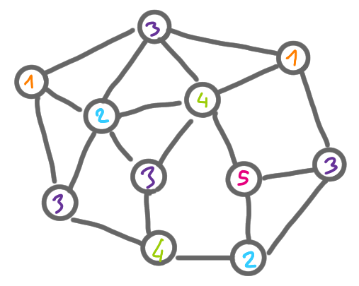
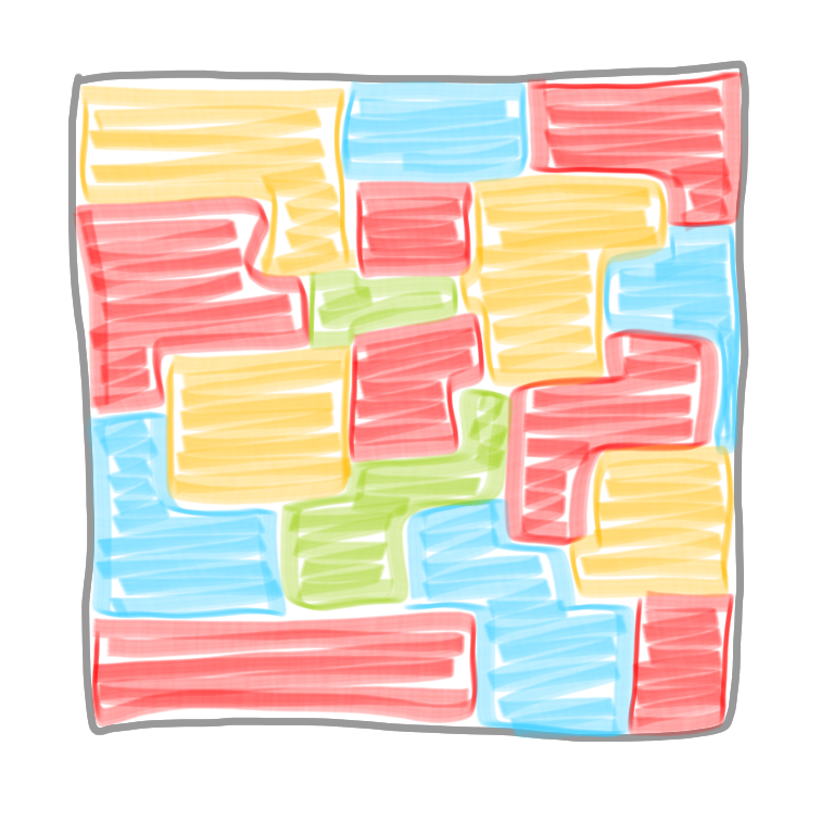
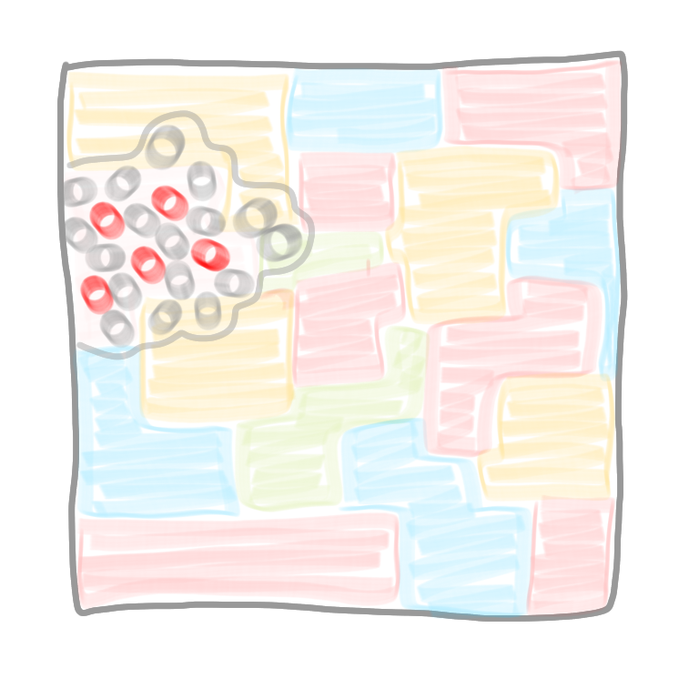
In a network decomposition, instead of having a coloring “at the level of the nodes” that is where every node has a color different from its neighbors, we will color clusters of nodes and have a coloring “at the level of the clusters”. In some sense we change scale. A network decomposition looks a bit like this.

Now there are three questions: What exactly is a network decomposition? How to use it? and How to compute it?

Definition of network decomposition

Definition A network decomposition with parameters $c$ and $d$ is a labeling of the nodes with colors from 1 to $c$, such that for any given color, the (maximal) connected components with this color have diameter at most $d$.

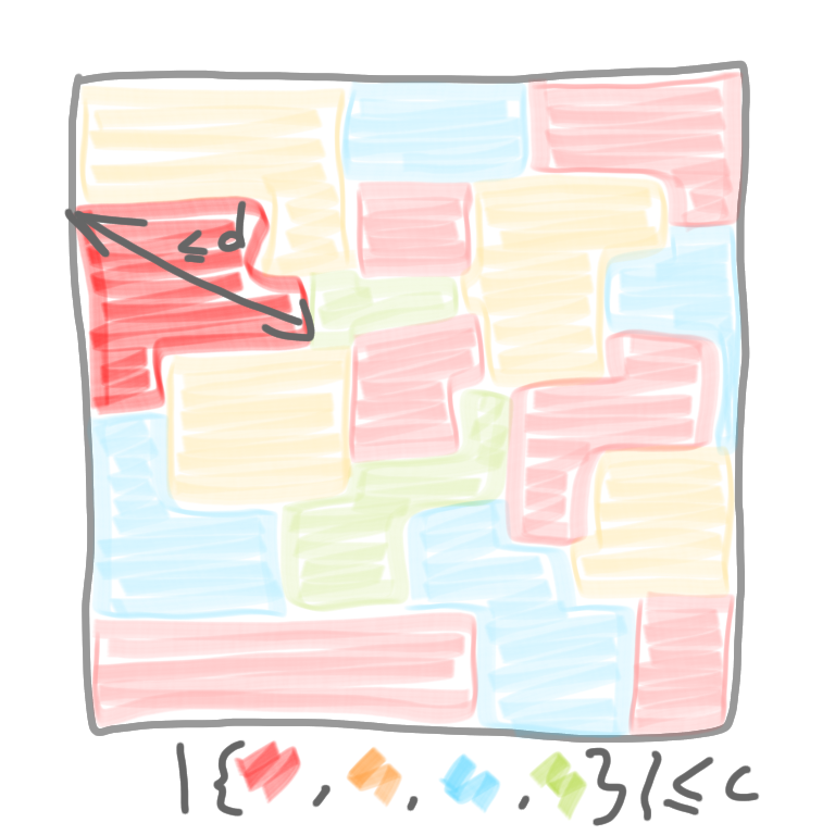
[There are some subtleties with the definition, but let’s wait a bit before looking into that.]

So for example a proper $k$-coloring is a network decomposition with parameter $d=1$ and $c=k$. Also it is easy to have a network decomposition with parameters $d=n$ and $c=1$: color all nodes with color 1. In all this series of posts, what we will look for is a decomposition where both parameters are (poly)logarithmic in $n$.

How to use it?

We cannot use the exact same strategy as when we had a proper coloring. Indeed, in a network decomposition several nodes of the same color can be adjacent, thus they cannot just wake up and select themselves. Now it’s useful to remember the last part of the previous post about a general algorithm to solve any problem in time $O(n)$. Basically this algorithm was doing the following: at any point in time, every node sends to its neighbors everything it knows about the graph so far. Then step by steps we have the following:

1. When it starts a node knows only its identifier, and it sends it to its neighbors.
2. Then it receives the identifiers of its neighbors, thus in some sense it knows the graph at distance one around itself: it knows its degree and the IDs of its neighbors.
3. Then the node sends this information to its neighbors, and it receives the analogue information from its neighbors. With this, it can reconstruct its neighborhood at distance 2. That is, it is exactly the same as if it could see at distance 2 in the graph.
4. Iterating this process, after $k$ steps all nodes know their neighborhoods at distance $k$.

In the proof of the general $O(n)$ algorithm, we iterated this process until every node could see all the graph. That is we waited for $D$ steps, where $D$ is the diameter of the graph (and then as $D \leq n$, we got the result). But this process can be useful even if we do not wait up to $D$ rounds, that is, even if the nodes do not see the whole graph.

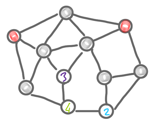
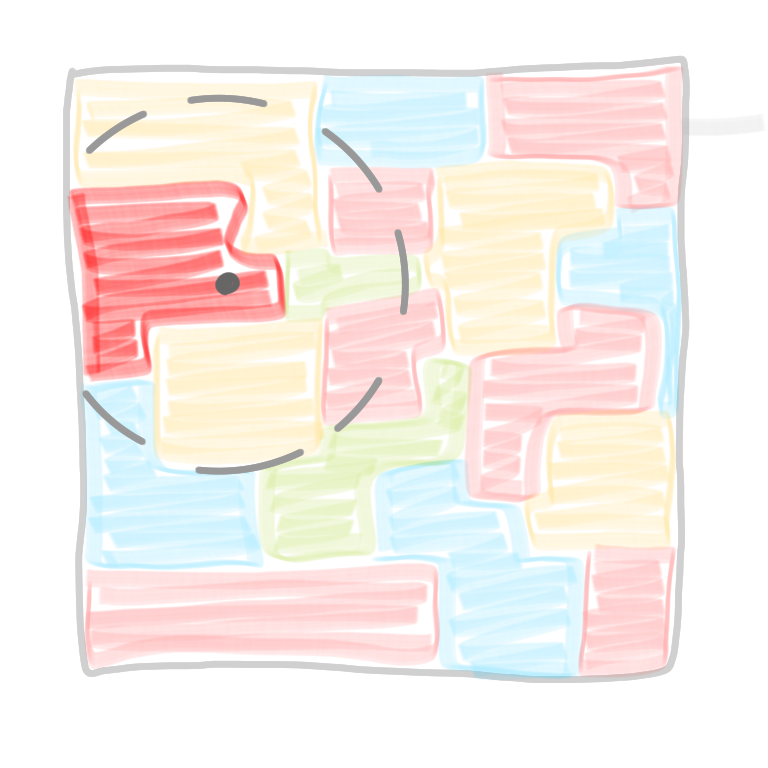
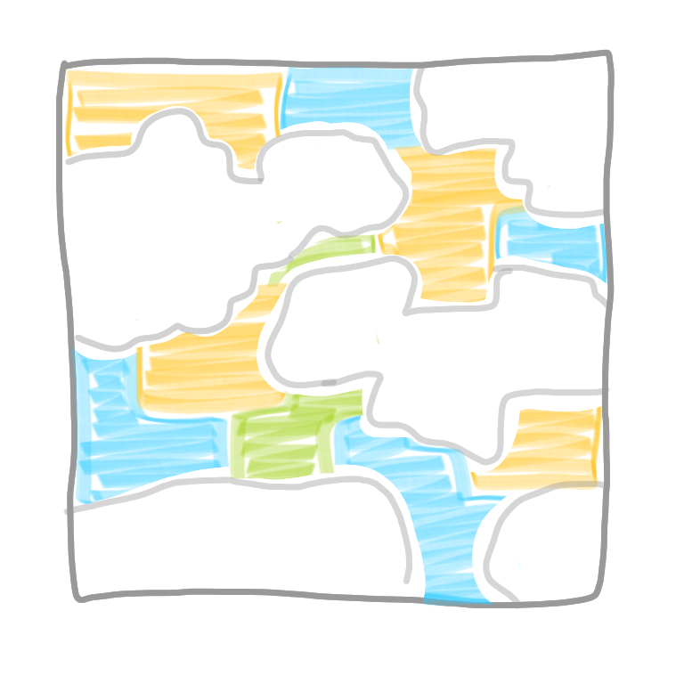
Given the network decomposition, let’s start by activating all the nodes of color 1. Now use the protocol above, for $d$ rounds. After this time, a node of color 1 knows all the nodes of its connected component. Indeed it can see at distance $d$ and we have been promised that the diameter of each connected component is at most $d$. Once this is done, we ask each node of the connected component to forget about the rest of the graph, to compute an MIS in what remains, and to output whether it is selected or not in this MIS. Note that it is exactly the same thing as what we did in the previous post but on a subgraph.

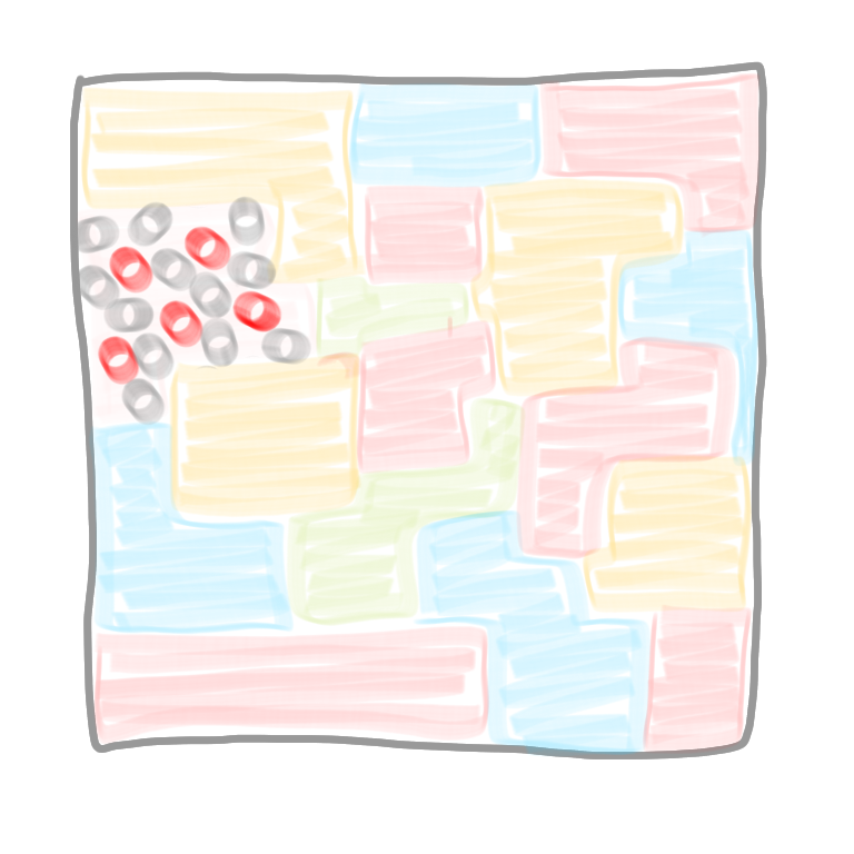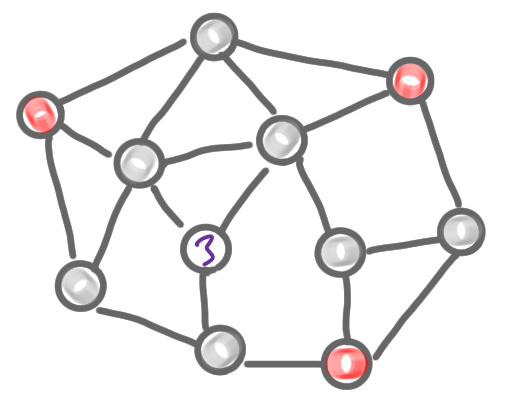
At the end of the phase, we have only selected and non-selected nodes in all the connected components of the first color. Note that these local MIS are correct, in the sense that there is no conflict: two connected components are necessarily non-adjacent (otherwise they wouldn’t be maximal). To finish this phase with the first color class, we de-select the nodes of the other color classes that are adjacent to a newly selected node of the first color class. After this step, all these nodes will not participate in the computation, and we can imagine that they are removed from the graph

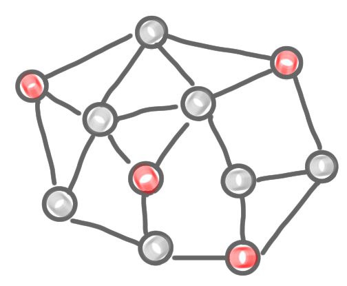
We can iterate this for all the color classes, just as we did when we had a proper coloring. Let us check the complexity. For each color we need the view at distance $d$, which takes $d$ rounds, and there are $c$ colors, so we have an algorithm in basically $d\times c$ rounds. In these posts, we look for a network decomposition with polylogarithmic parameters, such an decomposition gives us a polylogarithmic algorithm, which is awesome!

More generally

More generally, network decomposition is important and useful because it allows derandomization. More precisely, for a lot of classic problems, a polylogarithmic randomized algorithm is known, because randomization is a powerful tool to break symmetry. Now, with network decomposition it is possible to automatically transform these into deterministic polylogarithmic algorithms. See this paper for more inforamtion on this derandomization result.

Now we need to be able to build the network decomposition fast. This is the core topic of this series of posts.

Next post of the series: Centralized construction