Network decomposition 1: Local algorithms

09 Apr 2020

This the first real post of a series on distributed network decomposition. The introductory post of this series is here. This post is a quick introduction to local algorithms, with the example of the maximal independent set problem. If you have heard about the LOCAL model before, you probably know everything in this post.

A problem: computing a maximal independent set

A typical problem of network distributed computing is computing a maximal independent set (MIS). An MIS is a set $S$ of nodes of the graph such that no two nodes of $S$ are adjacent, and for every node not in $S$, there is neighbor in $S$.

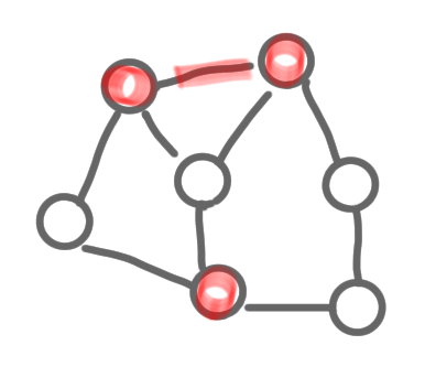
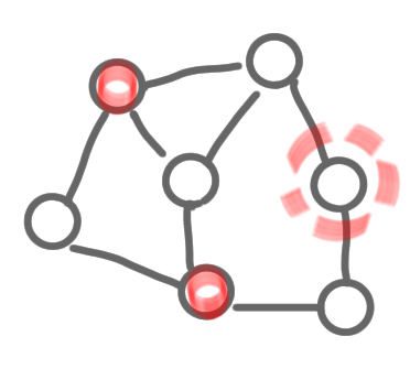
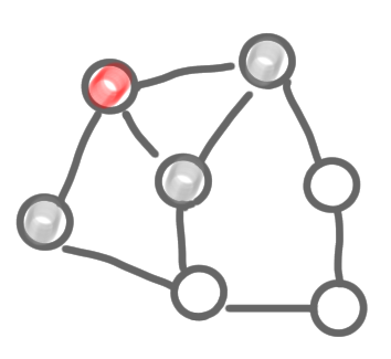
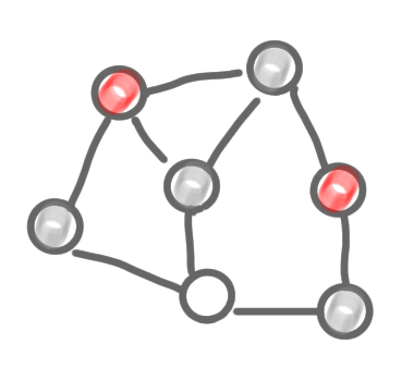
The two pictures below do not represent an MIS: the first one because of two adjacent selected nodes, and the second because of an “isolated node”.

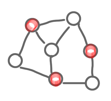
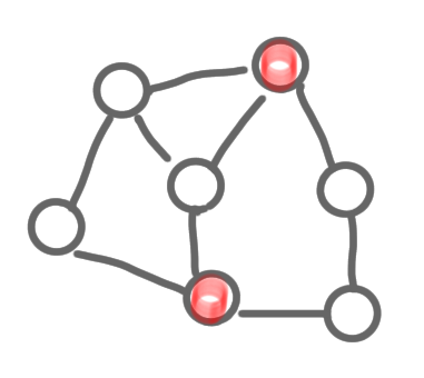
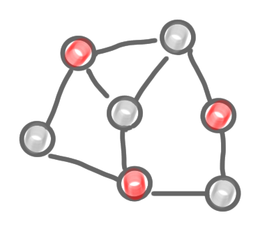
The two following pictures represent MISs. Note that one is maximum (it has 3 nodes, and no MIS on 4 nodes exists), but the other is just maximal, which is also fine.

Easy to solve in a centralized manner

It’s very easy to solve this problem in a centralized manner, in a greedy way. An algorithm is the following:

• Label all nodes as active
• As long as it is possible:

1. Take an arbitrary active node
2. Put it in the MIS
3. Label this node and all its neighbors as inactive

A first problem for us, with this algorithm, is that it is not distributed: you need an external entity to chose the “arbitrary active node”. This is some kind of scheduler, who decides which node is “doing something” at any step.

Using identifiers to simulate a centralized scheduler

In our model, we will assume that every node has a unique identity. This identifier is a number in $[1,n^2]$, where $n$ is the size of the netork (in general we take a large enough polynomial for the upper bound, but for concreteness let’s say $n^2$). For a node $v$, let $ID(v)$ be its identifier.

Using these identifier we will simulate the centralized scheduler.

All nodes start at the same time, and follow time steps (time-step= 1, 2, 3 etc. ). They start with a status that is active. The following algorithm is run at all nodes.

• If time-step = $ID(v)$ and status = active:

1. Change status to selected
2. Send message “selected” to all neighbors

• If the time-step $\neq ID(v)$ and status = active:

1. Wait for a message “selected” from neighbors
2. If one arrives, change status to not selected

One can check that on our example, with the identifier given above, the run of the algorithm simulates the run of the centralized algorithm. Another identifier assignment would correspond to another centralized scheduler, and would give another MIS.

Note that the algorithm is correct because the identifiers are all distinct. Indeed, if two neighbors had the same identifier, they would be selected at the same time, and the outcome would not be an MIS.

Now to evaluate the performance of a local algorithm, we measure the number of time steps before the solution is completed. Here it is $n^2$ in general, as one would have to wait for the node with the largest identifier. This is a very poor complexity. Indeed we finish this post with a proof that any problem can be solved in $O(n)$ time steps.

General algorithm in $O(n)$ steps

Consider the following algorithm (that is described partially by the pictures below).

• Send identifier to all neighbors
• Receive the identifier of all neighbors, and build the list of the adjacent edges, e.g. $(ID(v),ID(w))$ for a node $v$ receiving a message from a neighbor $w$.
• Send these edges to all neighbors.
• For $n$ time steps: send the set of all the edges received so far.
• Then build a local copy of the graph, solve the problem on this copy, and output the part of the solution that correspond to the node.

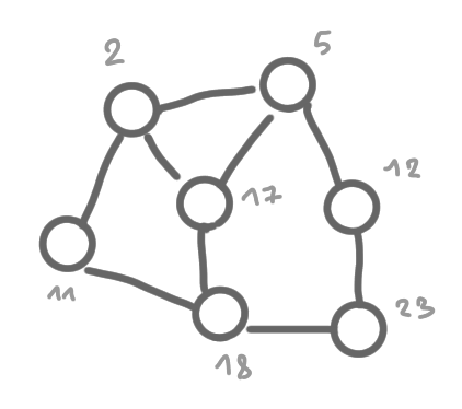
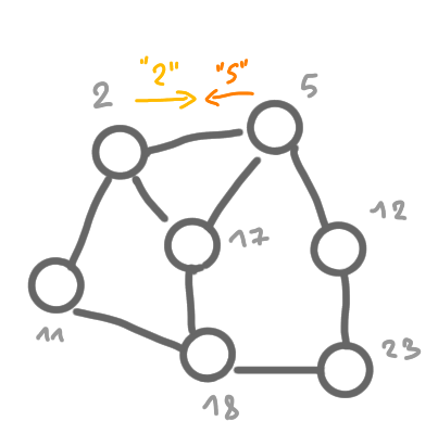
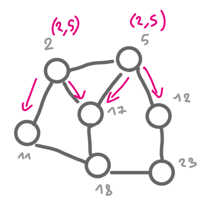
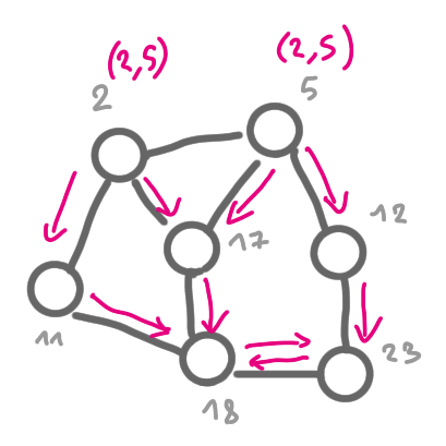
The following set of pictures shows how the information about the existence of the egde (2,5) is built and then broadcasted to the whole graph.

This algorithm is correct because after $n$ steps of flooding, all nodes know about all the edges, thus the local copy of the graph that each node has is correct, and then the output of the algorithm is also correct.

Next post of the series: Impact on distributed algorithms