SSS 2020 report 2: Compression of programmable matter
26 Nov 2020I continue the series about SSS 2020 that started here. (Again: I’m trying to not delay too much the publication of these posts so they won’t be very deep nor polished. Comments are most welcome.)
Austin's skyline. (The conference was supposed to be in Austin.)
Andrea Richa gave a nice keynote talk about programmable matter. The video is here.
Programmable matter is basically the idea that if you have many many very simple robots, then you can do interesting things, for example you can make them assemble into complicated useful shapes, or make them modify their environment in a way that a more classic robot would not be able to achieve. The talk featured (or “features” as the video is on the Internet) several interesting sections: a tour of the various ways to approach, design and use programmable matter, a theoretical approach to a specific problem, and the way the designed theoretical solution can be adapted to fit the “real world conditions”. For this post I’ll focus on the second part (which is based on this paper), but the two other ones are very interesting too, and I really enjoyed the discussion of back-and-forths between theory and practice.
The model and the problem
The model is the following. You have a large number of identical robots on a triangular grid (theoretical models for programmable matter often use such girds but in reality there’s not always such an underlying structure.) Every node can basically see the six positions around itself, and check whether they are occupied by robots or not. And every robot can move to these neighboring positions if it does not already contain a robot.
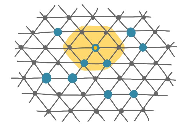
A set of blue robots. The one highlighted by a yellow dot can see and move to the positions in the yellow region.
Now there is a million of model variations that you can consider, playing with what the robots can see, what they can compute, what they know about the environment, and when they can move (synchronous/asynchronous etc.). But let’s not go into details here.
The problem we’ll consider for these robots is called compression. Before describing it let’s define a graph: there is one node for each robot, and an edge between any two adjacent robots.
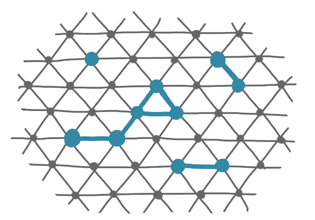
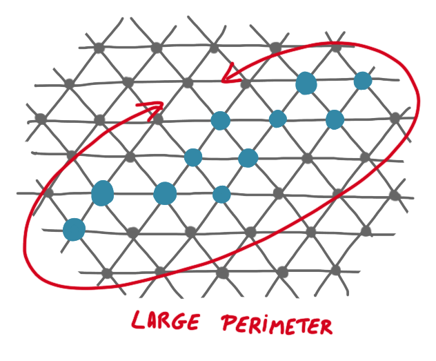
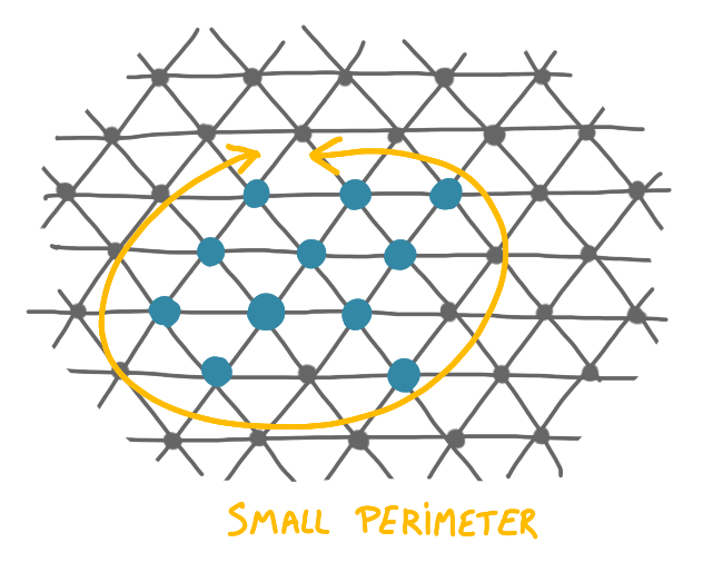
For the compression problem, you start from a situation where the set of robots is connected (in the sense that the graph is connected) but still scattered in the grid, and you want to gather them together as tighly as possible. One measure of the compression would be the diameter of the configuration, but we use the perimeter instead, which is technically more handy. Note that the perimeter is also a natural measure of compression: the disc is the shape that has the best compression, and it has the smallest perimeter.
As finding a minimum perimeter is a hard task, one considers a relaxation, which consists in looking for an $\alpha$-compressed solution, which is simply a configuration where the perimeter is at most $\alpha$ times the minimum perimeter.
Algorithm idea
The first intuition to have is that having a small perimeter is the same as having a large number of edges in the induced graph. (Andrea says it’s easy to prove.) Then one can naturally try to make the robots move in a greedy manner to a position that maximizes the number of edges locally.
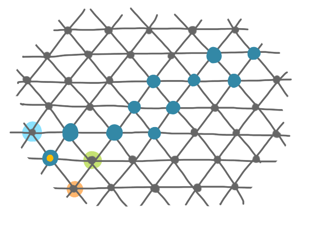
On this picture, the robot with the dot has several adjacent positions with diverse "quality": the blue position has the same number of edges as the current position (1 edge), the orange position is even worse (0 edge), and the green one is better (2 edges).
Now, the authors use a kind of randomized version of this that can sometimes move to a position with a lower degree. One reason for this is to avoid local minima. (You can see that on the picture above, no node except the one I chose could actually move if one insists on movements that strictly improve the situation.) They consider a model where at each time step a particle is chosen uniformly at random, then this particle selects an adjacent position (occupied or not) uniformly at random, and if the position is unoccupied, it considers whether to move to this position or to stay at its current position. The robot moves from position $p_1$ to the adjacent (unoccupied)position $p_2$, with probability \(\min(1,\lambda^{\Delta_2-\Delta_1})\), where $\lambda>1$ is a real number to be fixed latter, and $\Delta_i$ is the degree of the robot in position $i$. Thus, if the other position considered strictly improves the degree, the robots always moves and otherwise it might move, but it might also stay at the same position.
There are some additional topics around connectivity and holes, and around replacing the uniform scheduling of the robots by something more local, but again, let’s not go into that.
Results
It is possible to prove that the random process described by the algorithm is a Markov chain that converges to a stationary distribution, and that the probability of a distribution is proportional to $\lambda^E$, where $E$ is the number of edges in the induced graph. As a consequence, one can then get with very high probability an $\alpha$-compressed configuration (with some relation between the probability and the $\alpha$).
Getting to a stationary distribution is not proven to be fast (the best upper bounds are exponential), but simulations show that one gets a compressed configuration in polynomial time. One thing to note here is that one can actually get to an $\alpha$-compressed configuration much before stabilization, so this discrepancy is not that surprising.
A surprising phenomenon in the algorithm above is the following: if you chose $\lambda$ high enough (say larger than 4), then you get the behavior described above, but if you chose it smaller (say between 1 and 2), then you can prove that the configuration does not compress but expand! More precisely with such small $\lambda$ (but still larger than 1), at the end you have configuration whose perimeter is at least a fraction of the maximum perimeter.