A research story about patterns in graphs (1)
09 Sep 2020Almost one year ago, I wrote a blog post about graph classes and patterns, and said that some other posts would follow. Well, there has not been no other posts, but now the paper has been definitely accepted in a journal so it’s a good moment to write about this again. Actually, I won’t continue on the purely scientific perspective of the first post, instead I’ll tell the story of the paper. I really enjoy such “research stories”, and unfortunately they are not often told.
Starting point
The story begins in Chile where I did an internship in 2013 with José Correa. When I arrived, José had just attended IPCO (which had been organized in Valparaiso), and came back with a problem we could study. The problem is following.
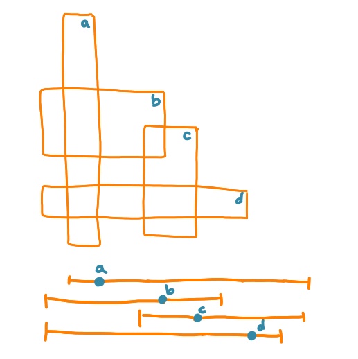
Input: A set of axis-aligned rectangles touching some curve.
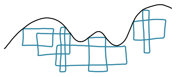
Task: Find the maximum independent set of rectangles.

I think I remember the paper was presenting an approximation algorithm with a large approximation ratio, and anyway it was not the main focus of the authors (but to be honest I don’t remember).
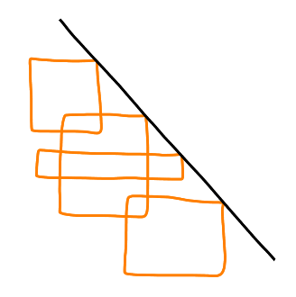
After some quick research, it appeared that the general problem of maximum independent set of rectangles (without the curve) was a popular one, thus worth studying even in special cases. The idea was to simplify it even more than in the IPCO paper and to try to have a clean approximation algorithm with a small approximation ratio. We ended up studying configurations where the curve is a decreasing straight line.
Some results
After some time, we basically had two results: a polynomial-time exact algorithm for this case, and a characterization of the intersection graph. Here the intersection graph is defined by creating a node for each rectangle and having an edge when the two corresponding rectangles intersect
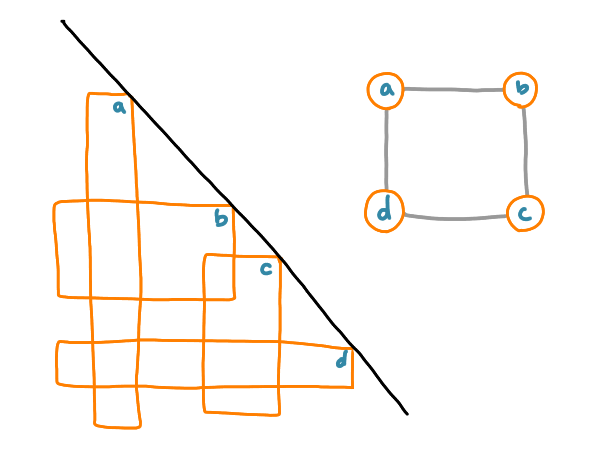
The characterization is the following: a graph is the intersection graph of rectangles intersecting a diagonal line (that we called diagonal rectangle graphs) if and only if there exists an ordering of the nodes such that the following pattern does not appear: four nodes $a< b < c < d$, such that $(a,c)$ and $(b,d)$ are edges and $(b,c)$ is not an edge.
It is easy to see that, if you consider the ordering of the rectangles along the diagonal, it is not possible to have some rectangles $A$, $B$, $C$ and $D$ in this order, such that $A$ and $C$ intersect, and $B$ and $D$ intersect, but $B$ and $C$ do not intersect.

It is not much harder to prove the full characterization.
First twist and sensors
Then I gave a talk at the local seminar about these results, and someone in the audience asked “How long have you been working on that? Because we have been working on the exact same graphs.” It was Mauricio Soto who was working 200 meters away from my office. He and Christopher Thraves had been working on the graph class (and not the optimization problem) for some time, and ended up with the same characterization. What is funny is that they came from a completely different path.
Mauricio and Chirstopher were interested in sensor networks. A classic model for those, is to consider that you have some sensors in the plane, and that every sensor can communicate with the other sensors that are at distance at most $d$ (where $d$ is some parameter).
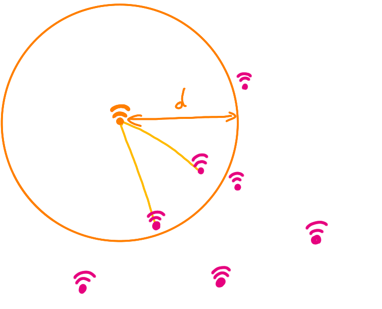
Now you can associate a graph with this model: a node for each sensor, and an edge every time two sensors can communicate.
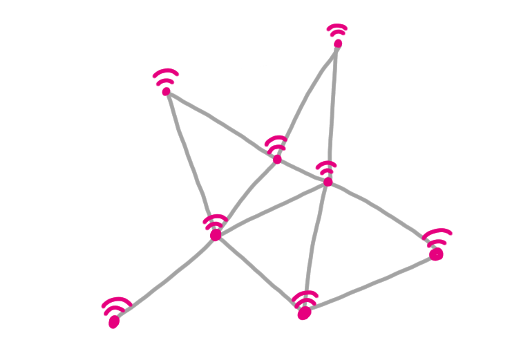
This is equivalent to consider the intersection graph where you have a disks of radius $d/2$ around each sensor, and put an edge if the disks intersect.
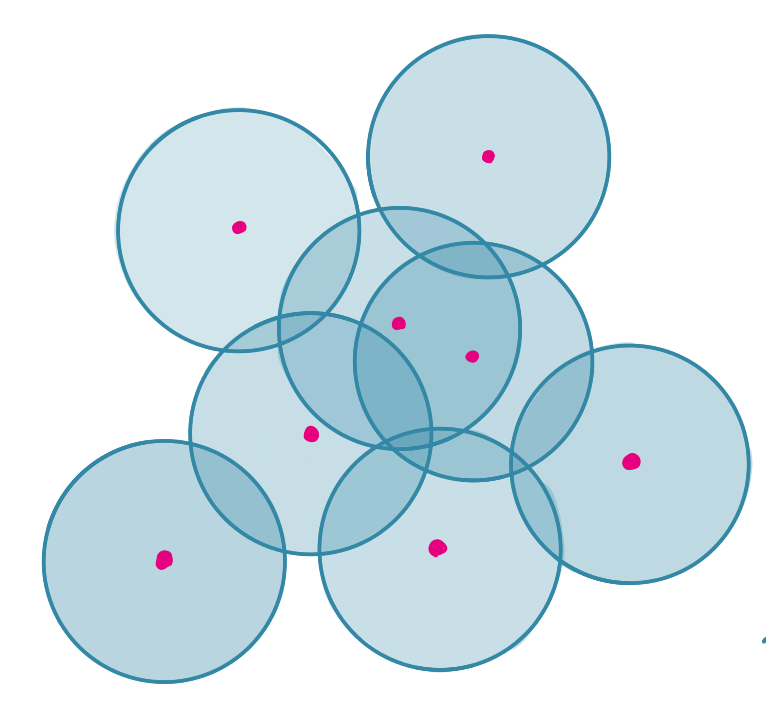
And as we can re-scale everything, we can say that $d/2=1$ and the class of graphs is called unit disk graphs.
Now what Mauriocio and Christopher were after was a class of graphs that could handle the cases where the sensors do not have the same range in every direction (because of technology issues or obstacles) and are not identical. As this is a pretty wild scenario, they decided to start with the case where the sensors are aligned. Now every sensor has a position on the line and an interval that represent the zone it can “see”. The graph that they associate with this case is the intersection graph where two sensors “intersect” if they can see each other, that is if each sensor is in the interval of the other.
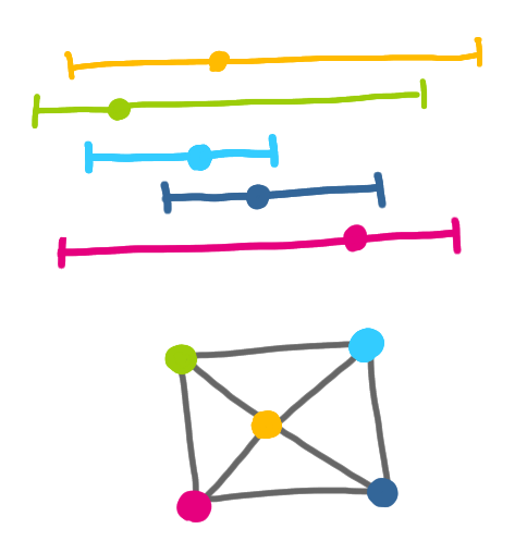
And now this class of graphs they call p-box graphs, ends up being the exact same class as our diagonal rectangle graphs! Basically if you take the branch of the interval that is on the right to the sensor point and make it vertical, you can create a rectangle.
In the end, their work was more on the graph theory aspects and ours more on the optimization side, so we decide not to merge the results, and to continue on our respective paths (acknowledging the other group in the future papers).
Notes
- The paper by Mauricio and Christopher.
- Thanks to Fabien Dufoulon for spotting some typos.