Simulation argument II. Edge-labelings on 2-colored trees, and polynomials

12 Feb 2019

This is the second post of a series that starts here.

---

---

In the previous post, we saw an overview of the simulation technique. In this post, we are going to see a more precise and usable approach, for the case of edge labelings on 2-colored regular trees.

The explanation differs a bit from the original paper, because we talk about polynomials, whereas they talk about regular expressions. This is mainly a vocabulary change, because there is not much algebra going on (but it is easier for me to see it this way).

A restricted setting

Let us describe the special case we are interested in, and why it is relevant.

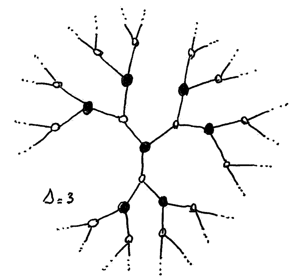
$\Delta$-regular trees

We consider that we are in the middle of a $\Delta$-regular tree. Here “middle” means that we cannot see the leaves. As a consequence, the method works only for the regime below time $\Theta(\log n)$, because in time $\Omega(\log n)$ you can always see a leaf in a $\Delta$-regular tree. If we can prove a lower bound for this area of the tree, then we have a lower bound for our problem.

2-coloring

We will consider graphs that are 2-colored (trees are bipartite), and we assume that every node knows on which side of the partition it is (black or white). So we work on this kind of graph (with omitted port-numbers):

This, in addition to port-numbers, is a powerful way to break symmetry between adjacent nodes.¹

A white algorithm in $k$ rounds for a problem $\Pi$ is an algorithm such that, after $k$ rounds the white nodes label their edges in a correct way, with respect to $\Pi$. In such an algorithm, the black nodes do not label the edges, they “trust” the white nodes. A black algorithm is defined the same way, but for black nodes.

Encoding of edge problems

Using the 2-coloring

We consider edge problems defined the following way. The multiset of edges adjacent to any vertex should follow some rule, that depends on the color of the node. For example: there are three labels $a,b,c$, the white nodes should either have 2 edges labeled with $a$, and the rest with $c$, or 3 edges labeled with $a$ and the rest with $b$; and black nodes should have at least one label $a$, one label $b$ and one label $c$. (I just made up this example, it’s probably silly.)

Most problems we are usually interested in are defined in general graphs, not in bipartite graphs, thus the problem does not refer to a coloring. Hence one could expect the constraints on white nodes and black nodes to be the same, unlike in the example above. Actually, it is often useful to make them different (we’ll see that in the two next posts).

Polynomial point of view

We now introduce the polynomial point of view. Consider a node $u$ in a graph where the edges are labeled. We can define the product of the labels of $u$ as a polynomial $M_u$, whose variables are the labels of the problem. Note that $M_u$ is a monomial: it’s just a product of labels.

One can now express the toy problem above in terms of two polynomials:

• $L_W(a,b,c)=a^2c^{\Delta-2}+a^3b^{\Delta-3}$
• $L_B(a,b,c)=abc(a+b+c)^{\Delta-3}$

For two polynomials $P$ and $’$, let us denote by $P \subseteq P’$, the fact that the monomials of $P$ are all present in $P’$. Then the labeling of $u$ is correct for problem $\Pi$, if and only if, $M_u \subseteq L_{C(u)}$ (where $C(u)$ is the color of $u$).

Note that, in our example, all the polynomials we play with have three variables, because there are three labels, and that they are homogeneous of degree $\Delta$, because every node has $\Delta$ adjacent edges.

Simulation step and independence

Polynomial point of view

In the previous post, we said that the simulation step is basically about having a view at distance $T-1$, imagining everything that could appear in the nodes at distance $T$, and labeling edges with all the labels that could be correct in one of these extensions.

Now let us restate this in terms of polynomials. After the simulation, every edge is labeled with a set of labels. In term of polynomial, we represent such a set by a sum. Then the polynomial associated with a set labeling at a node $u$ could be for example $P_u=(a+b)^3(a+b+c)^4c^{\Delta-7}$, which means that three edges are labeled with $a$ and $b$, four edges are labeled with $a$, $b$ and $c$ and the rest is labeled with only $c$. (This polynomial would not work for our toy language as we will see later).

Note that the polynomial corresponding to set labeling is not a monomial in general, for example $P_u$ is not. But this polynomial is nevertheless in a factorized form.

Simulation for 2-colored trees

For 2-colored trees, we can be more specific in the description of the simulation (and actually we will change the simulation outline a bit).

We have a white algorithm in time $T$, and we want a black algorithm in time $T-1$ (this will be our setting until the end of the post). Consider a black node $u$. The black node $u$ will first imagine all the extensions of its $(T-1)$-view into a $(T+1)$-view. (Note that we simulate at distance $T+1$ and not just $T$, as stated in the previous post.) The black node will then simulate the run of its white neighbors with the algorithm in time $T$, and gather the set of labels possible for each edge.

Note that we have fixed the topology to $\Delta$-regular trees, so the only thing to imagine for the extension is the port-number assignment.

Independence

The key point here is the following: the $T$-view of a white neighbor $v$ of $u$ consists of: (1) the $(T-1)$-view of $u$, and (2) the extension of this view in the direction of $v$. In the following picture, this means that this view includes only the black part and the red part.

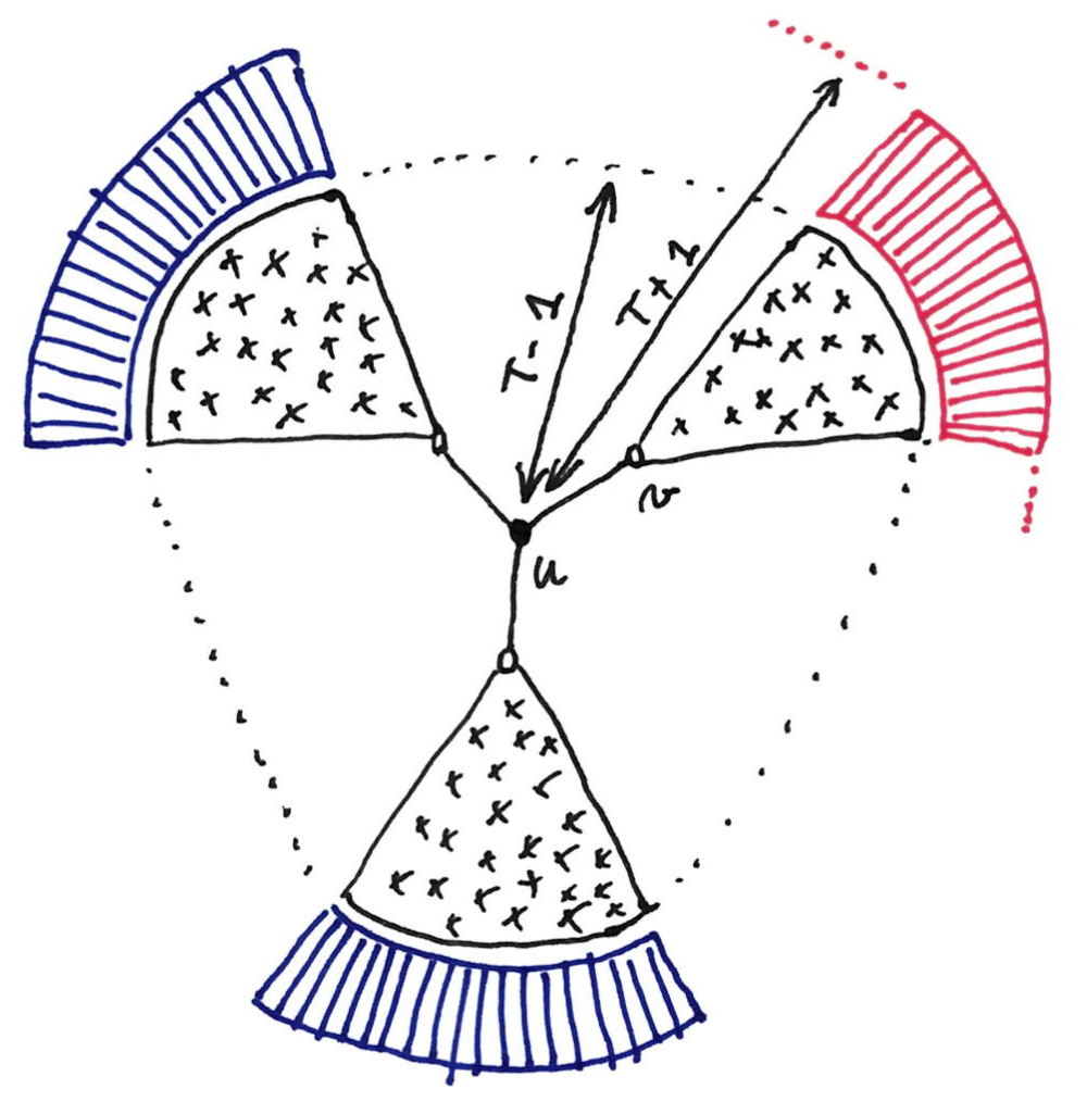
As a consequence when simulating node $v$, the black node does not need to imagine something for the other parts of its imaginary $(T+1)$-view (e.g. the blue parts on the figure). In other words the labeling of the edge $(u,v)$ comes only from the different version of the red part, and is independent of what happens in the blue parts. Obviously this independence property is true for every white neighbor of $u$, with its “own” extension.

Two key properties

We now describe two properties of set labelings coming from simulations, that will be essential for deriving lower bounds.

Product property

This property is about the neighborhood of the black nodes.

Claim: Let $S_1, S_2, …, S_{\Delta}$ be the sets of labels that a black nodes gives to its adjacent edges after the simulation step (with an arbitrary order of the edges). Then any tuple of the form $(s_1, s_2,…, s_{\Delta})$, with $s_i\in S_i$, has to be in the language (for the black side).

Proof: Suppose it is not the case, and let $(s_1, s_2,…, s_{\Delta})$ be a tuple of $S_1, S_2, …, S_{\Delta}$ that is not in the language. Then we build an extension such that the $T$-round algorithm would label the edges with $(s_1, s_2,…, s_{\Delta})$, which is a contradiction with the correctness of the algorithm. Start with $s_1$. If $s_1$ is in $S_1$ it means that there is an extension, in the direction of the first edge (in the figure, suppose $(u,v)$ is the first edge, then we are talking about the red part), such that the first edge is labeled with $s_1$, and we take this extension. But, because of the independence property stated above, we can continue with $s_2$, and then $s_3$ etc., which leads to the desired structure.

We can restate this in terms of polynomials.

Product property: $P_u \subseteq L_B$.

This means that every monomial of $P_u$ has to be a monomial of $L_B$, which is just a reformulation of the claim above.

Consistency property

Note that during the simulation, different edges around a white node have been labeled by different black nodes. Thus, a priori, the set labels on these edges are rather uncorrelated: they come from different simulations, based on different local views of the graph. Nevertheless, the following claim says something about the set labels around a white node.

Claim: Consider a set labeling around a white node after simulation. For each edge one can select a label in the set, such that the resulting labeling around the white node is correct for the language $L_W$.

Proof: Consider the original white algorithm in time $T$, and run it on the graph. The resulting labeling is correct for both black and white nodes. We claim that after the simulation, on every edge, the set of labels contains the label given by this $T$-round white algorithm. Indeed, one of the extension imagined by the black node for simulation is the real extension, therefore the corresponding label appears in the set. Thus the claim.

Typical transformation step

The typical way to prove that one has a transformation from an algorithm in $T$ rounds for a problem $\Pi$, to an algorithm in $T-1$ rounds for a problem $\Pi’$, is the following.

First make the simulation. In our example, we know that the black node $u$ gets a polynomial included in $(a+b+c)^{\Delta}$. But this is a very rough over-approximation, and $P_u$ is probably much smaller. Then one can use the two key properties to rule out many labelings and have a more precise idea of what $P_u$ is. Once this is done, we can go for a simplification step: replace sets of labels by simple labels. If everything works fine you have a labeling that is correct for your problem $\Pi’$.

Choosing the problems $\Pi$, $\Pi’$ etc., and designing the right simplification steps is the core of a proof by simulation.

Subtleties

There are two subtleties that blocked me at some point.

The first one is that the simulation performed by different nodes have to be handled carefully. For example, one could try to use the simulation to set-label more edges basically all the edges around a white node). This is very dangerous, and it seems much better to focus only on the edges around the black node at hand.

The second is that in this 2-colored framework, it is not enough to have a general way to go from a white $T$-round algorithm to a black $(T-1)$-round algorithm, you also need to go from a black algorithm to a white algorithm. In some cases, the two are very different.

Footnotes